Contents
Soccer and Machine Learning: 2 hot topics
I’m sure you’ve probably heard about the 2018 FIFA Football World Cup in Russia everywhere during the last few months. And, if you are a techy, I guess you also have realized that Machine Learning and Artificial Intelligence are buzzwords too. So, what better way to start off this 2018 than by writing a post that combines these two hot topics in a machine learning tutorial! In order to do that, I’m going to leverage a dataset of the Fifa 2018 video game.
My goal is to show you how to create a predictive model that is able to forecast how good a soccer player is based on their game statistics (using Python in a Jupyter Notebook). Fifa is one of the most well known video games around the world. You’ve probably played it at least once, right? Although I’m not a fan of video games, when I saw the dataset collected by Aman Srivastava, I immediately thought that it was great for practicing some of the basics of any Machine Learning Project. The Fifa 18 dataset was scraped from the website sofifa.com containing statistics and more than 70 attributes for each player in the Full version of FIFA 18. In this Github Project you can access the csv files that compose the dataset and some jupyter notebooks with the python code used to collect the data. Having said this, now let’s start!
Getting started with the machine learning tutorial
In our recently published Machine Learning e-book we explained most of the basic concepts related to smart systems and how machine learning techniques could add smart capabilities to many kinds of systems in almost any domain that you can imagine. Among other things, we learned that a typical workflow for a Machine Learning Project usually looks like the one shown in the image below:
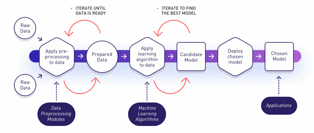
In this post we’ll go through a simplified view of this whole process, with a practical implementation of each phase. The main objective is to show most of the common steps performed during any machine learning project. Therefore, you could use it as a start point in case you need to address a machine learning project from scratch.
In what follows, we will:
- Apply some preprocessing steps to prepare the data.
- Then, we will perform a descriptive analysis of the data to better understand the main characteristics that they have.
- We will continue by practicing how to train different machine learning models using scikit-learn. It is one of the most popular python libraries for machine learning. We will also use a subset of the dataset for training purposes.
- Then, we will iterate and evaluate the learned models by using unseen data. Later, we will compare them until we find a good model that meets our expectations.
- Once we have chosen the candidate model, we will use it to perform predictions and to create a simple web application that consumes this predictive model.
At the end, we will arrive at a funny smart app like the one below. It will be able to predict how good a soccer player is based on their game statistics. Sounds cool, yeah? Well, let’s dive in!
1. Preparing the Data
Generally any machine learning project has an initial stage known as data prepapration, data cleaning or the preprocessing phase.
Its main objective is to collect and prepare the data that the learning algorithms will use during the training phase. In our practical and concrete example, an important part of this was already addressed by Aman Srivastava when he scraped different pages from the website sofifa.com. In his Github Project you can access some of the jupyter notebooks with the python code that acts as the data preprocessing modules that were applied to get and generate the original dataset for our project. Below, as an example, we can see the module that does the web scraping of the raw data (html format) and how it transforms the data into a Pandas dataframe (Pandas is a famous Python library for data processing). Finally it generates a csv file with the results. In some way, this data preparation step can be seen like something similar to the old ETLs (extract, transform, load) database processes.
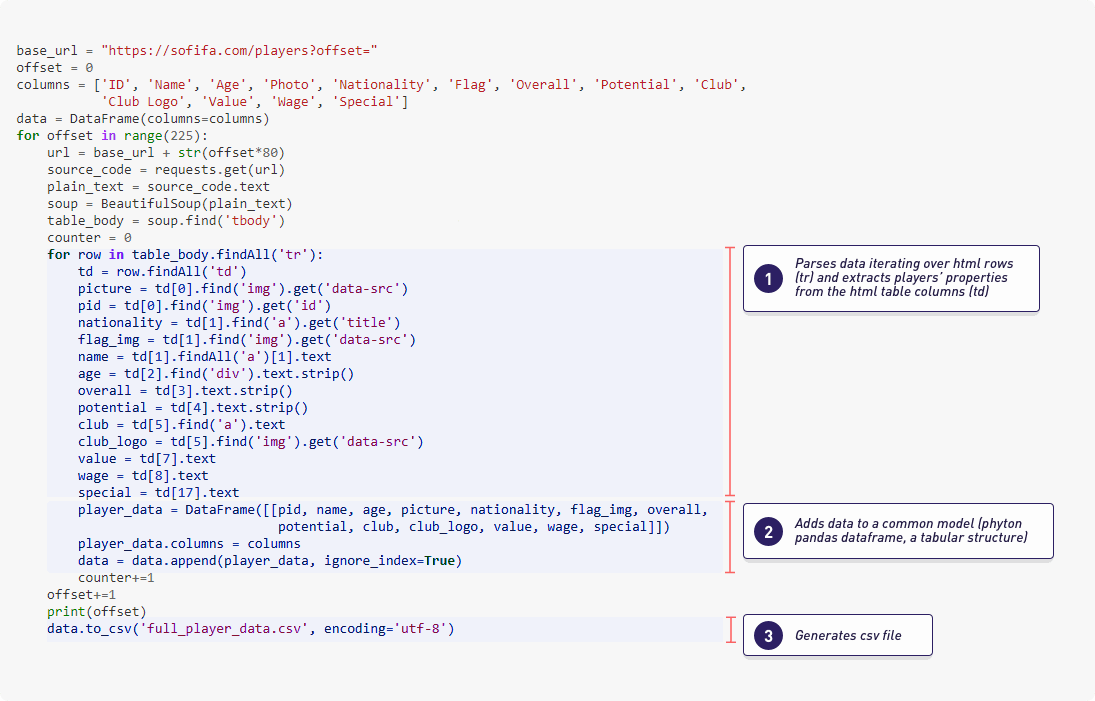
Python Preprocessing module from crawler.ipynb
Many times, multiple sources need to be consumed to collect relevant data for our algorithms. The problem is that different sources have different data quality, different formats, languages, units, etc.
Common issues that we generally face during the data preparation phase:
- Format and structure normalization
- Detect and fix missing values
- Duplicates removal
- Units normalization
- Constraints validations
- Anomaly detection and removal
- Study of features importance/relevance
- Dimentional reduction, feature selection & extraction
Below, we can see an additional second python script that we added specifically for our project and it continues the pipeline of the preprocessing phase. It takes the complete dataset from the merged CompleteDataset.csv file and it applies some cleanup (anomaly removal) and additional transformations (units normalization) to the data for some of the initial features (columns) that we are going to use. The
Overall column refers to a player’s current rating/ability. That’s what we are going to use as a measure of how good the player is. We will consider Overall as the observable dependent variable that we want to understand. After learning how it relates to the player’s characteristics (also known as features, predictors or independent variables which explain the dependent value), we will predict the results. In order to keep it simple, for now we will avoid any automated dimensional reduction techniques to select the most relevant features of a player. We’ll follow our instincts and common sense to choose Value column as a good feature from where to start. Besides, we can easily imagine there’s a high relation between the value that a player has in the market and how good this player is. Later we will add other features like the age or how good the player is at finishing to try to improve our predictors.
Take a look:
|
1 2 3 4 5 6 7 8 9 10 11 12 13 14 15 16 17 18 19 20 21 |
import numpy as np # Linear algebra import pandas as pd # Data processing col_types = {'Overall': np.int32, 'Age': np.int32} #read only the columns that we will use (name and photo are loaded only to visualize the results at the end) df = pd.read_csv("CompleteDataset.csv", usecols=['Name', 'Photo', 'Value', 'Overall', 'Age', 'Finishing'], dtype=col_types) #remove € character, leave just numbers df['Value'] = df['Value'].str.replace('€', '') #parse string for millions and thousands to numeric values def parseValue(strVal): if 'M' in strVal: return int(float(strVal.replace('M', '')) * 1000000) elif 'K' in strVal: return int(float(strVal.replace('K', '')) * 1000) else: return int(strVal) df['Value'] = df['Value'].apply(lambda x: parseValue(x)) |
|
1 2 |
#check if there are null/missing values and how many in each column df.isnull().sum() |
|
1 2 3 4 5 6 7 |
Name 0 Age 0 Photo 0 Overall 0 Value 0 Finishing 0 dtype: int64 |
Great!
We can see that we do not have null or missing values. If we had, then we could remove them before continuing. To complete this phase we are going to look for anomaly entries. For instance, we know that nobody could have a value in the market lower than or equal to zero. So those values are bad entries and we need to remove them since they could be dangerous, causing overfitting (an undesirable characteristic of any machine learning model).
|
1 2 |
#Nobody can have a value lower or equal than zero, so those values are bad entries and we need to remove them df = df.loc[df.Value > 0] |
Also, we have observed that there are a few non-numeric entries in the Finishing column, so we are going to exclude them.
|
1 2 3 4 5 6 7 8 9 10 11 12 |
def between_1_and_99(s): try: n = int(s) return (1 <= n and n <= 99) except ValueError: return False #remove not valid entries for Finishing df = df.loc[df['Finishing'].apply(lambda x: between_1_and_99(x))] #now we can define Finishing as integers df['Finishing'] = df['Finishing'].astype('int') |
We could continue executing many other validations and transformations to the data, for instance, check that all values in the Overall column are in the range between 0 and 100, that there are no duplicated entries, etc. But, remember that this is a simplified view of a typical workflow of a machine learning project because we simply want to demonstrate the fundamental ideas today.
Let’s see how our data looks in the first few rows:
|
1 |
df.head() |
| Name | Age | Photo | Overall | Value | Finishing | |
|---|---|---|---|---|---|---|
| 0 | Cristiano Ronaldo | 32 | https://cdn.sofifa.org/48/18/players/20801.png | 94 | 95500000 | 94 |
| 1 | L. Messi | 30 | https://cdn.sofifa.org/48/18/players/158023.png | 93 | 105000000 | 95 |
| 2 | Neymar | 25 | https://cdn.sofifa.org/48/18/players/190871.png | 92 | 123000000 | 89 |
| 3 | L. Suárez | 30 | https://cdn.sofifa.org/48/18/players/176580.png | 92 | 97000000 | 94 |
| 4 | M. Neuer | 31 | https://cdn.sofifa.org/48/18/players/167495.png | 92 | 61000000 | 13 |
If you find some other interesting preprocessing steps, go ahead! We encourage you to practice with Python and Pandas and let us know how it goes!
Expert corner:
If you are starting with this kind of project I strongly recommend you to use the Anaconda distribution which simplifies the whole installation of the most popular and important packages to work with big-data projects, data-science projects and predictive analysis.
Some important packages included in the Anaconda distribution:
- NumPy
- SciPy
- Matplotlib
- Jupyter
- Scikit-learn (the library that we will use later in this post when creating the predictive models)
Some good IDEs to start with are:
- Spyder (included in Anaconda)
- Jupyter Notebook (we actually used it for this post!)
- Python Tools for Visual Studio (I personally like it very much)
So, take a look at them and choose the one suitable for you and that you’re comfortable with!
1.1 Understanding the data
Now that the data is ready, before we start applying machine learning algorithms, a good approach is to first explore, play with, and query the data to get to know it better. This process is known as
descriptive analysis. The main objective here is to have a very good understanding of our data. It means to understand the kind of distribution it has and get some statistics, among others. If you skip this phase, you’ll feel like you’re on a blind date with it later. So, let’s explore the data and get to know what we’re working with!
|
1 |
df.describe() |
| Age | Overall | Value | Finishing | |
|---|---|---|---|---|
| count | 17611.000000 | 17611.000000 | 1.761100e+04 | 17611.000000 |
| mean | 25.106013 | 66.229175 | 2.417993e+06 | 45.256487 |
| std | 4.602144 | 7.003240 | 5.392879e+06 | 19.447567 |
| min | 16.000000 | 46.000000 | 1.000000e+04 | 2.000000 |
| 25% | 21.000000 | 62.000000 | 3.250000e+05 | 29.000000 |
| 50% | 25.000000 | 66.000000 | 7.000000e+05 | 48.000000 |
| 75% | 28.000000 | 71.000000 | 2.100000e+06 | 61.000000 |
| max | 44.000000 | 94.000000 | 1.230000e+08 | 95.000000 |
As you can see above, by using the describe operation provided by any Pandas dataframe we can get a summary of some important properties of our data like:
- the number of rows (a.k.a observations)
- average values
- minimums and maximums
- percentiles’ values
- standard deviation
This operation can be applied to the whole dataframe or you can select particular features, for instance, if you want to see statistics only for the Overall feature you can do it in this way:
|
1 |
df.Overall.describe() |
|
1 2 3 4 5 6 7 8 9 |
count 17611.000000 mean 66.229175 std 7.003240 min 46.000000 25% 62.000000 50% 66.000000 75% 71.000000 max 94.000000 Name: Overall, dtype: float64 |
The Overall column refers to a player’s current rating/ability and since it’s the variable that we will use as a measure of how good or bad a player is, then we can get some initial interpretations of our data from the above statistics like the following statements:
- We have 17611 observations (players) under study
- The average player’s Overall value is about 66
- The worst player has an
Overall value of 46 - The best player has an
Overall value of 94 - Only one quarter of the players have an
Overall value greater than 71
Right now I’m a bit curious to know about who are the best and worst players.
Let’s see who they are by querying our data.
|
1 |
df.nlargest(5, columns='Overall') |
| Name | Age | Photo | Overall | Value | Finishing | |
|---|---|---|---|---|---|---|
| 0 | Cristiano Ronaldo | 32 | https://cdn.sofifa.org/48/18/players/20801.png | 94 | 95500000 | 94 |
| 1 | L. Messi | 30 | https://cdn.sofifa.org/48/18/players/158023.png | 93 | 105000000 | 95 |
| 2 | Neymar | 25 | https://cdn.sofifa.org/48/18/players/190871.png | 92 | 123000000 | 89 |
| 3 | L. Suárez | 30 | https://cdn.sofifa.org/48/18/players/176580.png | 92 | 97000000 | 94 |
| 4 | M. Neuer | 31 | https://cdn.sofifa.org/48/18/players/167495.png | 92 | 61000000 | 13 |
|
1 |
df.nsmallest(5, columns='Overall') |
| Name | Age | Photo | Overall | Value | Finishing | |
|---|---|---|---|---|---|---|
| 17973 | T. Sawyer | 18 | https://cdn.sofifa.org/48/18/players/240403.png | 46 | 50000 | 35 |
| 17974 | J. Keeble | 18 | https://cdn.sofifa.org/48/18/players/240404.png | 46 | 40000 | 15 |
| 17975 | T. Käßemodel | 28 | https://cdn.sofifa.org/48/18/players/235352.png | 46 | 30000 | 40 |
| 17976 | A. Kelsey | 17 | https://cdn.sofifa.org/48/18/players/237463.png | 46 | 50000 | 5 |
| 17978 | J. Young | 17 | https://cdn.sofifa.org/48/18/players/231381.png | 46 | 60000 | 47 |
Another thing that could be helpful when understanding the data is to see its distribution and try to figure out if it fits some well-known theoretical distribution. In order to do that, histograms can give us a good idea of the underlying data distribution. What they basically do is split the possible values/results into different bins and count the number of ocurrences (observations) where the variable under study falls into each bin. We can do this easily by using matplotlib, one of the most popular Python libraries for 2D plotting.
|
1 2 3 4 5 6 7 8 |
import matplotlib.pyplot as plt plt.hist(df.Overall, bins=16, alpha=0.6, color='y') plt.title("#Players per Overall") plt.xlabel("Overall") plt.ylabel("Count") plt.show() |
 This histogram probably reminds you of the bell shape that comes with a normal distribution. Normal distributions are very common when studying person’s traits (height, intelligence, etc). In this context, the concept of “normality” reflects the fact that the majority of the individuals have values near the mean. Similarly, it means that the number of individuals decreases quickly as soon as we go far from that mean. Let’s try to see how well our data fits a normal distribution. In order to do this, we can leverage the information provided previously when executing the describe operation, in particular the standard deviation property and the mean value. Let’s see those important values again:
|
1 2 3 |
overall_mean = df.Overall.mean() overall_std = df.Overall.std() print('The mean value for the Overall feature is ', overall_mean, ' and the standard deviation is ', overall_std) |
|
1 |
The mean value for the Overall feature is 66.22917494747601 and the standard deviation is 7.003240305890887 |
Let’s remember how the theoretical normal distribution looks and how the mean and standard deviation relate.

Source
Wikipedia
We can observe that the theoretical normal distribution is symetrical around the mean, that approximately 68% of the values fall between +/- 1 std from the mean, 95% fall between +/- 2 std from the mean and 99.7% fall betweeen +/- 3 std from the mean. As it’s explained in 68-95-99.7 rule, this rule can be expressed mathematically as follows:

Where X is an observation from a normally distributed random variable, μ is the mean of the distribution, and σ is its standard deviation. Previously, when describing the main properties of our data, we had observed that the 50th percentile was 66 and the mean was 66.2 making clear that half of the observations fall on each side of the mean, like in a normal distribution. Now, let’s see how the standard deviation meets the previous rule:
|
1 2 3 4 5 6 7 8 9 10 |
#number of observations in +/-1 std, +/- 2std and +/- 3 std std1_count = (df[(df.Overall >= (overall_mean - 1*overall_std)) & (df.Overall <= overall_mean + 1*overall_std)]['Overall']).count() std2_count = (df[(df.Overall >= (overall_mean - 2*overall_std)) & (df.Overall <= overall_mean + 2*overall_std)]['Overall']).count() std3_count = (df[(df.Overall >= (overall_mean - 3*overall_std)) & (df.Overall <= overall_mean + 3*overall_std)]['Overall']).count() #percentaje of observations in each range overall_total_count = df.Overall.count() percentage_std1 = std1_count/overall_total_count * 100 #empirically it should be 68% approx percentage_std2 = std2_count/overall_total_count * 100 #empirically it should be 95% approx percentage_std3 = std3_count/overall_total_count * 100 #empirically it should be 99.7% approx |
|
1 |
print('1 std % : ', percentage_std1, ', 2 std % : ', percentage_std2, ', 3 std % : ', percentage_std3) |
|
1 |
1 std % : 68.951223667 , 2 std % : 94.9236272784 , 3 std % : 99.8126171143 |
Nice! The Overall feature looks very normal!
In some way, this was expected if we think that it’s a property for which the concept of “normality” could apply perfectly (like other traits of a person, for instance height, weight, intelligence, etc). So, let’s confirm visually how well our data fits a normal distribution:
|
1 2 3 4 5 6 7 8 9 10 11 12 13 14 15 16 17 |
from scipy.stats import norm #plot the histogram plt.hist(df.Overall, bins=16, normed=True, alpha=0.6, color='g') plt.title("#Players per Overall") plt.xlabel("Overall") plt.ylabel("Count") # Plot the probability density function for norm xmin, xmax = plt.xlim() x = np.linspace(xmin, xmax, 100) p = norm.pdf(x, overall_mean, overall_std) plt.plot(x, p, 'k', linewidth=2, color='r') title = "#Players per Overall, Fit results: mean = %.2f, std = %.2f" % (overall_mean, overall_std) plt.title(title) plt.show() |
 Before ending this section, I’d like to highlight that sometimes the data preparation stage is underestimated (mainly when you are starting with your first machine learning projects) but you should know that this innocent-seeming first stage most of the time takes more than half of the total project time (sometimes even up to 60-80%!). So, keep that in mind and give this stage the importance it deserves.
2. Machine learning algorithms for building our predictive model
Now it’s time to create our predictive model. That is, to create a mathematical model which links our observed/dependent value/response (the Overall in our example) with the other features available (also called predictors or independent variables, like the Value column in this example). Machine Learning models are created during a learning phase, also known as the training process. As we described in our Machine Learning e-book, in its simplest form, the algorithms used to generate these models can be supervised or unsupervised (depending on their training mode).
In this case, we are working on a regression problem, and its algorithms fall in the supervised learning category (because we can train a model using observations where the expected result is well known and we can “teach” it to our algorithm). There are several algorithms that can be used to solve a regression problem, like what we are about to see. But first, let’s split our dataset in two different subsets. This is a common technique where we choose part of the dataset (generally 80%) for training purposes and the rest (approximately 20%) is used later as unseen data to evaluate how good our model is.
There are also some other techniques like cross-validation that can be applied in order to help minimize overfitting that you can try. For that, you can take a look at this article that gives a nice introduction to the Train/Test split technique, cross-validation, and the overfitting issue. That said, let’s continue splitting our dataset. We can do this very easily by using a pre-built functionality in the module model_selection as follows:
|
1 2 3 4 5 6 7 8 9 |
from sklearn.model_selection import train_test_split train, test = train_test_split(df, test_size=0.20, random_state=99) xtrain = train[['Value']] ytrain = train[['Overall']] xtest = test[['Value']] ytest = test[['Overall']] |
Since it’s reasonable to think that there could be a linear relationship between a player’s market value and how good they are, then we can create an initial model applying linear regression, one of the simplest regression models.
2.1 Linear Regression
For this and also for the rest of the models that we will see in this post, I’m going to use scikit-learn, a popular package for Python that provides implementations for most of the state-of-the-art machine learning algorithms that are usually used. So, we can train a default linear regresion model using scikit-learn with just a couple of lines of code as follows:
|
1 2 3 4 |
# Create linear regression object from sklearn import linear_model regr = linear_model.LinearRegression() regr.fit(xtrain, ytrain) |
|
1 |
LinearRegression(copy_X=True, fit_intercept=True, n_jobs=1, normalize=False) |
As you can see, we use the fit method to train our model. We just need to pass the independet features (xtrain) and the dependent values for them (ytrain). Later we will see that the same approach is used by scikit-learn to train different kinds of models. You’ll love scikit-learn because of this. This tool allows you to change and train different models using always a common approach and similar code. Now, we can use the already trained model and the predict method (that is also available for other kinds of predictive models) to predict how good the players in the test-set are. Remember that we split and reserved 20% of the hole dataset for evaluation/testing purposes it and was not part of the training process.
A good model should be able to understand generic hidden patterns in the data and also work well for unseen data.
|
1 2 |
# Make predictions using the testing set y_pred = regr.predict(xtest) |
Now let’s plot the line that represents our linear model!
We will do that to handle the predictions and also the real expected values that we know.
|
1 2 3 4 5 |
plt.scatter(xtest, ytest, color='black') plt.plot(xtest, y_pred, color='blue', linewidth=3) plt.xlabel("Value") plt.ylabel("Overall") plt.show() |
 At first glance, it may seem like this model is not very good 🙁 But, in case we can accept a model that produces a few bad predictions, with the most of them being good, then this model is not as bad as we thought. That’s because the predictions seem to be pretty accurate for those players with a value lower than €30M. Although it can not be appreciated very well in the plot, those players represent 99.33% of the total!
|
1 |
print('% of players with a value lower that €30M: ', df[df.Value <= 30000000].Value.count() / df.Value.count() * 100, '%') |
|
1 |
% of players with a value lower that €30M: 99.3299642269 % |
We can also visualize a histogram that shows the number of players in different ranges of values. It’s easy to see that most players have a value lower than €10M and it’s almost insignificant the amount of players with a value greater than €30M.
|
1 2 3 4 5 |
plt.hist(test.Value) plt.title("#Players per Value") plt.xlabel("Value") plt.ylabel("Count") plt.show() |
 At this point, you’re probably thinking that having some metric to represent how good our model is would be fantastic.
If so, you are right!
There are different metrics to evaluate this, for regression models two of the most common are the mean square error (MSE) and the r2 score. In general, we will want low values for the MSE and high values for the R2. That said, let’s use them and see the numbers for our model
|
1 2 3 4 5 6 7 8 |
import numpy as np # Linear algebra from sklearn.metrics import mean_squared_error, r2_score #common metris to evaluate regression models # The mean squared error print("Mean squared error: %.2f" % mean_squared_error(ytest, y_pred)) # Explained variance score: 1 is perfect prediction print('Variance score: %.2f' % r2_score(ytest, y_pred)) |
|
1 2 |
Mean squared error: 28.88 Variance score: 0.41 |
Now it’s time to decide whether this model is good enough for an initial app prototype. If it’s not the case, you will identify other algorithms and techniques to see if you can improve the initial model. In what follows, we will practice with some other techniques just in order to illustrate a general machine learning project workflow. With this objective, we will train a Ridge regression model to approximate the model’s function through polynomial interpolation and then an SVR model that is also a common option for nonlinear models.
2.2 Polynomial interpolation and Ridge Regression
If you’re familiar with calculus, you’ll know that a common and efficient way of computing a complex function is by approximating it by using polynomials. So, we can take this idea and assume that the data points in our dataset are points of a complex math function. Our goal is to find a polynomial that fits the curve of that function quite well. In linear regression models, we can use a trick known as basis functions that allow us to model nonlinear problems in terms of something linear. The trick consists in transforming the basic model of linear regression for a feature’s vector X = (x1,…,xn) from something like this ![]() into something like this
into something like this
![]()
You can note that the basic model is actually a special case of the general case when
![]()
What is really interesting about the previous transformation is that we can use a nonlinear function, and the model itself is still a linear model (because the coefficients never multiply or divides each other).
Now let’s move this math to code!
In this case, we’ll use polynomials as our basis functions and the Ridge model to solve the regression problem. Using Ridge regression (instead of the standard linear regression model) can help minimize overfitting, which is a possible colateral issue of adding basis functions to our regression model.
|
1 2 3 4 5 |
from sklearn.preprocessing import PolynomialFeatures from sklearn.pipeline import make_pipeline pol = make_pipeline(PolynomialFeatures(6), linear_model.Ridge()) pol.fit(xtrain, ytrain) |
I decided on the value, 6, for the degree parameter after doing some manual experimentation with the parameters. If you have some time, I recommend you can give a quick overview about hyper-parameters optimization phase for finding the best values that can be configured when training a model.
|
1 2 3 4 5 6 |
y_pol = pol.predict(xtest) plt.scatter(xtest, ytest, color='black') plt.scatter(xtest, y_pol, color='blue') plt.xlabel("Value") plt.ylabel("Overall") plt.show() |
 Visually, the polynomial regression looks better than the standard linear regression. Like before, let’s see how good this model is by calculating the MSE and R2 metrics.
|
1 2 3 4 5 |
# The mean squared error print("Mean squared error: %.2f" % mean_squared_error(ytest, y_pol)) # Explained variance score: 1 is perfect prediction print('Variance score: %.2f' % r2_score(ytest, y_pol)) |
|
1 2 |
Mean squared error: 13.07 Variance score: 0.73 |
Very good! We have reduced MSE and increased R2 as we pretended 🙂
2.3 Support Vector Regression
The last model that we will try is called Support Vector Regression which can be seen as an extension of the Support Vector Machine method used for classification problems. In particular, we will use the SVR implementation (one of the three available implementations). Using the SVR implementation with a RBF (radial basis function) kernel is also a common approach for resolving nonlinear problems. We can define and train an SVR model with a RBF kernel as follows:
|
1 2 3 4 |
from sklearn.svm import SVR svr_rbf = SVR(kernel='rbf', gamma=1e-3, C=100, epsilon=0.1) svr_rbf.fit(xtrain, ytrain.values.ravel()) |
I’m leaving out of this explanation the different parameters for the SVR model. I defined the values above after a couple of manual experiments, but you could probably find a better combination. For now this configuration is good enough. In order to keep this simple we are not including a hyper-parameters optimization phase here. However, it’s something that you probably should do in a real project. Like for the previous models, we have the predict method available to get predictions:
|
1 |
y_rbf = svr_rbf.predict(xtest) |
Same as before, let’s plot both the real expected value and the predicted ones.
|
1 2 3 4 5 |
plt.scatter(xtest, ytest, color='black') plt.scatter(xtest, y_rbf, color='blue') plt.xlabel("Value") plt.ylabel("Overall") plt.show() |
 And following the same approach again let’s calculate the MSE and R2 metrics
|
1 2 3 4 5 |
# The mean squared error print("Mean squared error: %.2f" % mean_squared_error(ytest, y_rbf)) # Explained variance score: 1 is perfect prediction print('Variance score: %.2f' % r2_score(ytest, y_rbf)) |
|
1 2 |
Mean squared error: 6.00 Variance score: 0.88 |
This is really very good! We were able to considerably reduce the MSE and also increase the R2 score in an important way.
2.4 Adding more features to improve predictions
Let’s add now some more features to train our model. We are going to add the player’s age and how good the player is at scoring.
|
1 2 |
xtrain = train[['Value', 'Age', 'Finishing']] xtest = test[['Value', 'Age', 'Finishing']] |
|
1 |
xtrain.head() |
| Value | Age | Finishing | |
|---|---|---|---|
| 1141 | 12000000 | 23 | 76 |
| 13167 | 650000 | 19 | 55 |
| 17890 | 60000 | 18 | 43 |
| 5393 | 1400000 | 29 | 27 |
| 8268 | 550000 | 30 | 41 |
Let’s see if we can improve the models by using the new set of features as input:
Ordinary least squares regression using more features
|
1 2 3 4 5 |
regr_more_features = linear_model.LinearRegression() regr_more_features.fit(xtrain, ytrain) y_pred_more_features = regr_more_features.predict(xtest) print("Mean squared error: %.2f" % mean_squared_error(ytest, y_pred_more_features)) print('Variance score: %.2f' % r2_score(ytest, y_pred_more_features)) |
|
1 2 |
Mean squared error: 20.19 Variance score: 0.59 |
Polynomial regression using more features
|
1 2 3 4 5 |
pol_more_features = make_pipeline(PolynomialFeatures(4), linear_model.Ridge()) pol_more_features.fit(xtrain, ytrain) y_pol_more_features = pol_more_features.predict(xtest) print("Mean squared error: %.2f" % mean_squared_error(ytest, y_pol_more_features)) print('Variance score: %.2f' % r2_score(ytest, y_pol_more_features)) |
|
1 2 |
Mean squared error: 8.32 Variance score: 0.83 |
Support Vector regression using more features
|
1 2 3 4 5 |
svr_rbf_more_features = SVR(kernel='rbf', gamma=1e-3, C=100, epsilon=0.1) svr_rbf_more_features.fit(xtrain, ytrain.values.ravel()) y_rbf_more_features = svr_rbf_more_features.predict(xtest) print("Mean squared error: %.2f" % mean_squared_error(ytest, y_rbf_more_features)) print('Variance score: %.2f' % r2_score(ytest, y_rbf_more_features)) |
|
1 2 |
Mean squared error: 1.23 Variance score: 0.97 |
As you can see, we were able to improve our model’s precision even more. But wait, it’s important to note here that you won’t always get better results by adding more and more features. Adding redundant information or features that do not provide any relevant information for our interest could end up decreasing the quality and accuracy of predictions by overfitting the model. It also makes the model more complex, with more time needed for training it.
Feature engineering techniques can help to choose good features for our models. The study of a feature’s importance or relevance, feature selection and feature extraction, and applying dimentionally reduction techniques are important things to consider to find an optimal set of features to use. Having said that, you can do an exercise! Try to add many more features to train these same models and see if you can improve them. Next, let’s use the Support Vector Regression (SVR) model using more features (value, age and finishing) as our best candidate model. Let’s calculate and add to the test dataframe (unseen data) the predictions and also the error percentage that they represent.
|
1 2 3 |
pd.options.mode.chained_assignment = None test['Overall_Prediction_RBF'] = y_rbf_more_features test['Error_Percentage'] = np.abs((test.Overall - y_rbf_more_features) / test.Overall * 100) |
At this point I’m a bit curious about who are the players with the highest error rates in the predictions.
Let’s query the results to take a look:
|
1 |
test[['Name', 'Age', 'Value', 'Overall', 'Overall_Prediction_RBF','Error_Percentage']].nlargest(15, columns='Error_Percentage') |
| Name | Age | Value | Overall | Overall_Prediction_RBF | Error_Percentage | |
|---|---|---|---|---|---|---|
| 9 | G. Higuaín | 29 | 77000000 | 90 | 74.356462 | 17.381709 |
| 10 | Sergio Ramos | 31 | 52000000 | 90 | 74.356462 | 17.381709 |
| 15 | G. Bale | 27 | 69500000 | 89 | 74.356462 | 16.453413 |
| 21 | A. Griezmann | 26 | 75000000 | 88 | 74.356462 | 15.504020 |
| 23 | P. Aubameyang | 28 | 61000000 | 88 | 74.419167 | 15.432765 |
| 20 | J. Oblak | 24 | 57000000 | 88 | 74.734834 | 15.074052 |
| 52 | T. Müller | 27 | 47500000 | 86 | 74.356462 | 13.538998 |
| 48 | Isco | 25 | 56500000 | 86 | 74.356462 | 13.538998 |
| 69 | Y. Carrasco | 23 | 51500000 | 85 | 74.356462 | 12.521809 |
| 77 | B. Leno | 25 | 34000000 | 85 | 74.690997 | 12.128238 |
| 30 | Thiago Silva | 32 | 34000000 | 88 | 77.808358 | 11.581411 |
| 105 | K. Manolas | 26 | 31500000 | 84 | 75.177893 | 10.502509 |
| 132 | T. Lemar | 21 | 38500000 | 83 | 74.356462 | 10.413901 |
| 17759 | K. Tokushige | 33 | 20000 | 51 | 56.037744 | 9.877930 |
| 57 | David Luiz | 30 | 33000000 | 86 | 77.895012 | 9.424404 |
As you can see, there are only 13 players in the test dataset (13 in 3523 players, 0.37%) with a predicted error rate greater than 10%. We can also take a look at the histogram for the error variable.
|
1 2 3 4 5 |
plt.hist(test.Error_Percentage, bins=16) plt.title("#Players per %error") plt.xlabel("%error") plt.ylabel("Count") plt.show() |
 It’s easy to see that most players have a predicted error rate lower than 2%. Besides, the amount of players with an error rate greater than 5% is almost insignificant. Let’s use now the trained model to make predictions for all the players in the complete dataset:
|
1 2 3 |
y_rbf_all = svr_rbf_more_features.predict(df[['Value', 'Age', 'Finishing']]) print("Mean squared error: %.2f" % mean_squared_error(df[['Overall']], y_rbf_all)) print('Variance score: %.2f' % r2_score(df[['Overall']], y_rbf_all)) |
|
1 2 |
Mean squared error: 0.61 Variance score: 0.99 |
The metrics have improved more still. In fact, it makes sense because we added data that was part of the previous training process.
3. Building the application
Just as an illustrative step, we are going to build now a simple web application. It will be able to search players and list them among their predictions so you can play a bit with the results of this experiment. This prototype has a main disadvantage. Unfortunately, it can only display predictions for players in this dataset and not for new players in case you know their features (value, age and finishing). The reason for this simplification is that we are not hosting the real model with a backend side. I just generated a Javascript model for now that fits a basic AngularJS application, with the code that you can download from this GitHub. The javascript model for the players was built by adding the prediction and error to the main dataframe.
Later we used the “to_json” method as follows:
|
1 2 3 4 5 6 7 |
#from IPython.html import widgets pd.options.mode.chained_assignment = None df['Overall_Prediction_RBF'] = y_rbf_all df['Error_Percentage'] = np.abs((df.Overall - y_rbf_all) / df.Overall * 100) jsonDf = df.to_json(orient='records') #widgets.HTML(value = ''' players = ''' + jsonDf) |
In a real project, a more realistic architecture for hosting, consuming and updating a predictive model should be considered. But for a prototype I believe this is good enough. So, here you have the prototype!
4. Where to go next?
A well-known recommended approach when someone present some results in any research is to try to replicate the results by yourself. By doing this you can understand better, validate, find errors and improve things. So, if you liked this post and you are starting with predictive analytics and machine learning I encourage you to install the recommended software and environment. Then, execute the provided code to get your own results. If you felt a bit concerned about the math and statistics involved, you can go through lot of available content on the web. There’re posts, videos, courses, books and others, such as:
- Complete Course on Linear Algebra by MIT
- Complete Course on Multivariable Calculus by MIT
- Mathematics at Khan Academy
- Full Cheatsheet on Probability
- Here, some other book resources are also recommended
In particular, I liked the approach given in the following chapters of the Deep Learning Book (Goodfellow-et-al-2016) that summarizes very well all the required background knowledge:
- Chapter 2 (Linear Algebra)
- Chapter 3 (Probability and InformationTheory)
- Chapter 4 (Numerical Computation)
- Chapter 5 (Machine Learning Basics)
Continue to explore:
- Relationship between machine learning and big data and how to perform distributed processing
- Performance and the usage of gpgpu to train models
- Hyper-parameters tuning/optimization
- Cross-validation approach
- Feature engineering, feature relevance, feature selection, and extraction
- Dimentionally reduction techniques
- Apply and compare other techniques for regression problems
- Use of categorical variables
- Cold start problem (how to start when no data is available)
- Deploy of trained models
- Maintenance and update of models
- System’s architecture
So, if you try any of these things, please share with us your experience 🙂
End notes
During this machine learning tutorial, we went through a simplified view of a typical ML process, like the one presented in the diagram “The Machine Learning Process” at the beginning of this post. We gave a practical implementation of each phase showing most of the common steps that are generally performed. We leveraged the raw data provided by sofifa.com and some modules for preparing the data created by by Aman Srivastava and then we added new modules to the pipeline to continue adapting the data to our needs.
While studying the characteristics of our data, we were able to get some relevant information like mean, standard deviation, percentiles, maximum, minimum, etc. Also, we observed that a normal distribution described pretty well the distribution of our data. In order to practice with regression problems, we created different machine learning models. Among them, there are linear regression, polynomial regression and supported vector regression.
We used python and scikit-learn, starting with just one feature (value) and then adding some new features for training the models (age and finishing features). We noticed that by adding new features to the model, we would not always have better results and we mentioned common approaches to address this problem like feature selection, extraction and dimensionality reduction. As evaluation metrics for regression models, we applied two of the most commons: the mean square error (MSE) and the R2 score. We were able to improve these metrics considerably when comparing the first basic model and the last one.
Let us know your experience!
At the end of this journey, we ended up with a good candidate model. We embedded in a pure front end AngluarJS web application that allows the user to search players. Also, it’s possible to compare how good the players are against the system’s predictions. Even if you are not Peter Brand in the film MoneyBall (I strongly recommend this movie based on a true story if you haven´t seen it yet), the final app is still helpful to practice your machine learning knowledge (or if you are thinking in develop a sport bet site!). You also might want to try it during the upcoming 2018 FIFA Soccer World Cup. Don’t forget to comment your results 🙂
Wondering how to apply machine learning to something other than soccer? Check out our experience using AI to help with the difficult task of story points estimation!
About us
UruIT works with US companies, from startups to Fortune 500 enterprises, as nearshore partner for project definition, application design, and technical development. Our Uruguay and Colombia-based teams have worked on over 150 design and development projects up to date.
Are you ready to make the leap in your software development project? Tell us about your project and let’s talk.