Contents
Use Machine Learning for Software Development Estimation
In this work, we will present some ideas on how to build a smart component that is able to predict the complexity of a software development task. In particular, we will try to automate the process of sizing a task based on the information that is provided as part of its title and description and also leveraging the historical data of previous estimations.
In agile development, this technique is known as story points estimation and it defers from other classic estimation techniques that predict hours because the goal of this software development estimation is not to estimate how long a task will take, but to predict how complex a task is.
Typically, this software development estimation process is done by agile teams in order to know what all the tasks are that the team can commit to complete in the next sprint, generally a period of 2 weeks. Based on previous experience in the past 2 or 3 sprints, they can know in advance the average amount of points they are able to complete and so, they take that average as a measure of the threshold for the next sprint. Then, during the estimation process (generally through a fun activity like a planning poker), each member of the team gives a number of points that reflects how complex they think the task is.
There is a set of tasks that the team has decided to be the “base histories” that are well-known tasks already labeled with their associated complexity (that the team has agreed on) and can be used later as a base for comparison. After each sprint, new tasks can be added to this list. With time, this list can collect several examples of tasks with different complexities that the team can use later to compare and estimate new tasks. Teams generally reach a high level of accuracy in their estimations after some time, due to the continuous improvement based on accumulated experience, collecting more and more software development estimations.
Generally, the mental process that each team member goes through when estimating a new task is:
- Based on his/her previous experience, he/she looks for similar tasks that they have done in the past
- He/she gives the same number of points that similar tasks have been assigned in the past.
- If there isn’t a similar task, he/she starts an ordered comparison from the least to the most complex tasks. The reasoning is something like this: “Is this task more complex than these ones?” If so, he/she moves on with the set of well-known base tasks in order of increasing complexity. This process is repeated until the new task falls in one of the categories of complexity. By convention, in case a new task looks more complex than size X but less complex than size Y (Y being the next size in order of complexity after X) the size assigned for the task’s estimation will be Y.
If we look at this process, we can find lots of similarities with a classic machine learning problem, where we have a task, T, that improves over time with experience, E, by a performance measure, P. In our case, T is the task of estimating/predicting the complexity of a new ticket (bug, new feature, improvement, support, etc), the experience, E, is the historical data of previous estimations and the performance measure, P, is the difference between the actual level of complexity and the software development estimation.
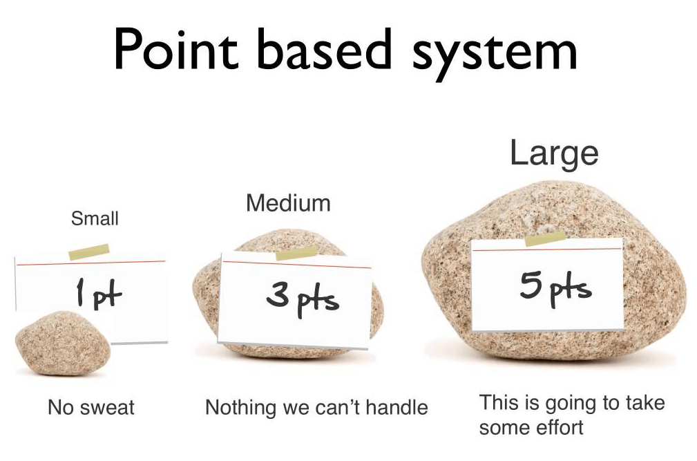
In the following, we present a machine learning approach to predict the complexity of a new task, based on the historical data of previously estimated tasks. We will use the Facebook FastText tool to learn text vector representations (word and sentence embeddings) that will be implicit used as input for a text classifier that classifies a task in three categories: easy, medium and complex. Note that we are changing things a bit, going from a point based estimation to a category based estimation.
This is because unfortunately, the number of estimates were very unbalanced in our dataset, and by grouping tasks into these three categories, we can slightly simplify our problem. Anyway, we can think of each of these classes (easy, medium, complex) as points in a simplified version of the story points estimation process (in a real story points estimation, size generally follows a Fibonacci sequence 1, 2, 3, 5, 8, 13, 21, etc., or some minor variation of this sequence).
In the end, we will build a basic web application like the one below, that is able to use the model that we trained so you can see it in action. It will allow you to search and pick up stories from the backlog (testing set) so you can compare the team’s average software development estimation vs the AI estimation (to see the AI’s prediction vs the team’s, click the cards on the right side! ). Sounds cool, yeah? Well, let’s dive in!
Out[1]:
Having said that, now let’s start!
Preparing the data
Let’s start by loading the appceleratorstudio dataset
In [22]:
|
1 2 3 4 |
import pandas as pd import numpy as np df = pd.read_csv("appceleratorstudio.csv", usecols=['issuekey', 'title', 'description', 'storypoint']) |
In [23]:
|
1 |
df.isnull().sum() |
Out [23]:
|
1 2 3 4 5 |
issuekey 0 title 0 description 43 storypoint 0 dtype: int64 |
In [24]:
|
1 |
df = df.dropna(how='any') |
Now, let’s see how our data looks in the first few rows:
In [25]:
|
1 |
df.head() |
A very good approach is to take a look at the main characteristics of the data that you are going to be working on. In order to do this, we can use the describe operation available in any pandas dataframe:
In [26]:
|
1 |
df.storypoint.describe() |
Out[26]:
- the number of rows (a.k.a observations)
- average values
- minimums and maximums
- percentiles’ values
- standard deviation
Another good idea is to plot a histogram. A histogram can give us a good notion of the underlying data distribution. What it basically does is split the possible values/results into different bins and counts the number of occurrences (observations) where the variable under study falls into each bin. We can do this easily by using matplotlib, one of the most popular Python libraries for 2D plotting.
In [27]:
|
1 2 3 4 5 6 7 8 |
import matplotlib.pyplot as plt plt.hist(df.storypoint, bins=20, alpha=0.6, color='y') plt.title("#Items per Point") plt.xlabel("Points") plt.ylabel("Count") plt.show() |

We can easily see that the number of occurrences is not uniform throughout the different size categories (points).
Let’s see the amount of items per point:
In [28]:
|
1 |
df.groupby('storypoint').size() |
Out[28]:
In our case, we will start by grouping points into three different categories to reduce the imbalanced data.
In [29]:
|
1 2 3 |
df.loc[df.storypoint <= 2, 'storypoint'] = 0 #small df.loc[(df.storypoint > 2) & (df.storypoint <= 5), 'storypoint'] = 1 #medium df.loc[df.storypoint > 5, 'storypoint'] = 2 #big |
In [30]:
|
1 |
df.groupby('storypoint').size() |
Out[30]:
At this point, it’s important to note that in this work the goal is to solve a classification problem (predict the class associated to the complexity of a task: 0-easy, 1-medium or 2-complex) instead of a regression problem (predict a continuous real value) like in the paper, A deep learning model for estimating story points.
Before we continue, let’s do some cleanup to our data. This is also a common step that generally any machine learning process needs to apply because of the following issues:
Common issues generally faced during the data preparation phase:
- Format and structure normalization
- Detect and fix missing values
- Remove duplicates
- Normalize units
- Validate constraints
- Detect and remove anomalies
- Study features importance/relevance
- Dimentional reduction, feature selection & extraction
For this work, most of these issues were already addressed by the authors of A deep learning model for estimating story points when collecting the dataset. Anyway, we will need to do some extra cleanup to the data for our purpose: remove some html tags as well English stop words (words like the, this, that, etc) because they can add noise to our problem and it’s better to remove them.
In [31]:
|
1 2 3 4 5 6 7 8 9 10 11 12 13 14 15 16 17 18 19 20 21 22 23 24 25 26 27 28 29 |
import numpy as np import csv from nltk.corpus import stopwords #Define some known html tokens that appear in the data to be removed later htmltokens = ['{html}','<div>','<pre>','<p>', '</div>','</pre>','</p>'] #Clean operation #Remove english stop words and html tokens def cleanData(text): result = '' for w in htmltokens: text = text.replace(w, '') text_words = text.split() resultwords = [word for word in text_words if word not in stopwords.words('english')] if len(resultwords) > 0: result = ' '.join(resultwords) else: print('Empty transformation for: ' + text) return result def formatFastTextClassifier(label): return "__label__" + str(label) + " " |
Important: Since we are removing stop words and html tags in our dataset, later when we want to predict with some unseen data we will need to apply the same transformation before requesting the model’s prediction for that input.
- One new column called “title_desc” that is just the concatenation of the title and description columns
- A second column called “label_title_desc” that contains the number of points with a specific prefix expected by FastText to recognize it as the labeled information (class)
While doing this, we will also change everything to lower case to make the training phase case insensitive. These new columns will be used later for training our learning algorithms.
In [32]:
|
1 2 |
df['title_desc'] = df['title'].str.lower() + ' - ' + df['description'].str.lower() df['label_title_desc'] = df['storypoint'].apply(lambda x: formatFastTextClassifier(x)) + df['title_desc'].apply(lambda x: cleanData(str(x))) |
In [33]:
|
1 |
df = df.reset_index(drop=True) |
Dealing with the imbalanced dataset – Oversampling
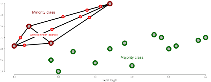
Other more complex oversampling techniques exist, like SMOTE, where artificial datapoints (called synthetic data points) are created by taking two datapoints in the minority class (one datapoint and one of its k nearest neighbors) creating the new artificial point in the space between the two real points. If we think about this technique in a 2D scenario, the new datapoint is created in some random place on the line between the two points as you can see in the image below:
Anyway, for this work, a basic oversampling technique that creates copies of the existing data was used. The main reason for that is simplicity, because dealing with new synthetic datapoint created artificially implies finding a text representation for a sentence that could map to that new vector representation, because in the end, the FastText tool expects text in sentences and not the embeddings. Possible workarounds exist for this like approximating the synthetic point with a new sentence generated by averaging the embeddings of words used by the nearest k sentences to the synthetic points, for instance. This could be something interesting to try, so if you do it please let us know your results!
Note: Basic random downsampling of the majority class that is also a common and simple technique was combined with the oversampling, but didn’t improve the results. So, in the end, just a basic oversampling was used in order to minimize the effect of an imbalanced dataset.
In [34]:
|
1 2 3 4 5 6 7 8 9 10 11 12 13 14 15 16 17 18 19 20 21 22 23 24 25 |
from collections import Counter def SimpleOverSample(_xtrain, _ytrain): xtrain = list(_xtrain) ytrain = list(_ytrain) samples_counter = Counter(ytrain) max_samples = sorted(samples_counter.values(), reverse=True)[0] for sc in samples_counter: init_samples = samples_counter[sc] samples_to_add = max_samples - init_samples if samples_to_add > 0: #collect indices to oversample for the current class index = list() for i in range(len(ytrain)): if(ytrain[i] == sc): index.append(i) #select samples to copy for the current class copy_from = [xtrain[i] for i in index] index_copy = 0 for i in range(samples_to_add): xtrain.append(copy_from[index_copy % len(copy_from)]) ytrain.append(sc) index_copy += 1 return xtrain, ytrain |
Creating our classifier
Without entering into much detail, we can say that embeddings consist of techniques that learn vector representations of words, sentences, or documents, so that the vector representation of similar and semantically related words, sentences, or documents are close together in the high dimensional vector space. Then, by leveraging this characteristic onto the learned vectors, we can use them as features for any kind of machine learning algorithm, to train a classifier or as input to a clustering algorithm, etc.
Word embedding techniques are not something new in Natural Language Processing (NLP), although in the last years, new embeddings techniques based in predictive neural networks models have become very popular and they have revolutionized the machine learning field in many domains, not just that of NLP. Word embeddings have started to be used in other domains like e-commerce and recommender systems with the variation known as prod2vec, meta-prod2vec, or in mobile applications like app2vec, among others. Recently, I’ve applied different embedding techniques to create Internet Domain Name embeddings from DNS trace logs and they have demonstrated to be a good approach for learning semantic similarities and analogy tasks between Internet Domain Names. You can see details about how I have used word2vec for learning Internet Domain Names in Vector representation of Internet Domain Names using a Word Embedding technique
FastText
In regard to FastText, its main advantage over word2vec is that it considers subwords inside a word. Instead of considering each word as a single token, a word is split into a set of substrings called ngrams and later the training phase is done considering each subword of a word, and the vector representation of a word is formed by averaging the vector representation of its subwords (and the word itself). The most important parameters to tune when using FastText are minn and maxn that define the min and max length of n-grams when splitting words.
Additionally, FastText can be used either in supervised or unsupervised mode. When using FastText in supervised mode, you can train a supervised model by using a dataset specially prepared (labeled) using a set of sentences (one per line) along with a label that acts as the class to which the sentence belongs. So, by training a FastText model in supervised mode, you can later perform classification tasks over new unseen sentences, which is very helpful for a lot of text classification and sentiment analysis problems.
Having said this, we present a simple custom python wrapper for the supervised mode of the native FastText interface. Although there is already a wrapper for FastText and a native module in the well-known Gensim package, none of them include support for the supervised mode of FastText (only the unsupervised mode). So, I decided to create our custom and very basic wrapper with the minimum that we need for our purpose, that is:
- a constructor to create new instances of the wrapper with its own state
- a fit method to trigger the training process by calling the executable file and passing the required parameters (*)
- a predict method that receives an array with a list of sentences and returns another array (of the same size) with the integer predictions in {0, 1, 2} for each sentence
(*) The training process is executed with the following parameters:
- 500 epochs (iterations over the corpus)
- Vector size of 300 dimensions
- minn=4 and maxn=6 (minimum and maximum numbers of n-grams respectively)
- pretrained file used to transfer previous knowledge of the English language and domain-specific knowledge (I’ve tried using the pretrained vectors for English language provided by FastText, but in the end generating my own pretrained models using other system datasets in the same domain worked better. You can download these other datasets from the same github repository in order to use them for building your own pre-trained model.
In [35]:
|
1 2 3 4 5 6 7 8 9 10 11 12 13 14 15 16 17 18 19 20 21 22 23 24 25 26 27 28 29 30 31 32 33 34 35 36 37 38 |
import uuid import subprocess class FastTextClassifier: rand = "" inputFileName = "" outputFileName = "" testFileName = "" def __init__(self): self.rand = str(uuid.uuid4()) self.inputFileName = "issues_train_" + self.rand + ".txt" self.outputFileName = "supervised_classifier_model_" + self.rand self.testFileName = "issues_test_" + self.rand + ".txt" def fit(self, xtrain, ytrain): outfile=open(self.inputFileName, mode="w", encoding="utf-8") for i in range(len(xtrain)): #line = "__label__" + str(ytrain[i]) + " " + xtrain[i] line = xtrain[i] outfile.write(line + '\n') outfile.close() p1 = subprocess.Popen(["cmd", "/C", "fasttext supervised -input " + self.inputFileName + " -output " + self.outputFileName + " -epoch 500 -wordNgrams 4 -dim 300 -minn 4 -maxn 6 -pretrainedVectors pretrain_model.vec"],stdout=subprocess.PIPE) p1.communicate()[0].decode("utf-8").split("\r\n") def predict(self, xtest): #save test file outfile=open(self.testFileName, mode="w", encoding="utf-8") for i in range(len(xtest)): outfile.write(xtest[i] + '\n') outfile.close() #get predictions p1 = subprocess.Popen(["cmd", "/C", "fasttext predict " + self.outputFileName + ".bin " + self.testFileName],stdout=subprocess.PIPE) output_lines = p1.communicate()[0].decode("utf-8").split("\r\n") test_pred = [int(p.replace('__label__','')) for p in output_lines if p != ''] return test_pred |
About pre-trained models
In our particular case, we base our predictions on understanding the meaning of the natural language information provided in the title and description of each entry. So, having a pretrained model of English text could be very helpful.
My first attempt was to use the pre-trained model available in the FastText Github repository for the English language. Although this improved the overall accuracy of my solution a bit, the improvement was not considered too much.
Deep Learning
The second approach that I followed was to use the same idea already applied in A deep learning model for estimating story points and use the pre-trained csv files (issues with title and description but without story points) in order to train a fastText unsupervised model in the same domain as my problem (software development issues) and use it later when training the fastText supervised classifier in my concrete problem and specific dataset. By doing this we can start with some basic knowledge, like vector representations for words and sentences in the software development domain (domain specific), so we can have a good parameter initialization without using the labeled data.
Using the second approach was much better than the first one (final results will be shown at the end). Although the pre-trained vectors trained from Wikipedia had been trained with considerably much more data than the pre-trained vectors that I got using the pre-trained csv files for other open source repositories, the second approach achieved the best results. This confirms something already known, that the use of pre-trained vectors trained in a similar domain can achieve better results even if they’re trained with much fewer data than other pre-trained vectors that were trained in a less similar domain.
The code below shows the files that were used to train the pre-trained vectors using other open source repositories and how to join them into a single pandas dataframe.
In [36]:
|
1 2 3 4 5 6 7 8 9 10 11 12 13 14 15 16 17 18 19 20 21 22 23 |
import pandas as pd import numpy as np pretrain_files = ['apache_pretrain.csv', 'jira_pretrain.csv', 'spring_pretrain.csv', 'talendforge_pretrain.csv', 'moodle_pretrain.csv', 'appcelerator_pretrain.csv', 'duraspace_pretrain.csv', 'mulesoft_pretrain.csv', 'lsstcorp_pretrain.csv'] pretrained = None for file in pretrain_files: df_pretrain = pd.read_csv('PretrainData/' + file, usecols=['issuekey', 'title', 'description']) if(pretrained is not None): pretrained = pd.concat([pretrained, df_pretrain]) else: pretrained = df_pretrain pretrained = pretrained.dropna(how='any') |
In [16]:
|
1 |
pretrained['title_desc'] = (pretrained['title'].str.lower() + ' - ' + pretrained['description'].str.lower()).apply(lambda x: cleanData(str(x))) |
In [17]:
|
1 2 3 4 |
outfile=open("issues_pretrain.txt", mode="w", encoding="utf-8") for line in pretrained.title_desc.values: outfile.write(line + '\n') outfile.close() |
fasttext skipgram -input issues_pretrain.txt -output pretrain_model -epoch 100 -wordNgrams 4 -dim 300 -minn 4 -maxn 6 -lr 0.01
Defining the training: an evaluation strategy
Selecting Training and Testing sets
Generally, we would like to have as much representative data as possible for training, and also a large number of different examples to put our model under test. But, sometimes it’s difficult to have both, mainly when we have small datasets like in our scenario. When this occurs, a technique called k-fold cross-validation can help us.
When using this approach, the data is split into k partitions (folds), then in each of the k iterations you select a different folder as the testing set and the rest of the folders are joined to create the new training set. In the end, an average evaluation cryteria of the k iterations is used to measure the quality of our model.
This is a common technique that helps evaluate models to ensure that the results do not depend on how you have selected your training data. K-fold cross-validation is also helpful when your dataset is small (like in our case), because you can ensure that every datapoint will be part of the training and also part of the testing set at any moment. Then, you do not risk leaving out of the training set some important (but few) examples like those that could occur if you use a fixed 80-20 approach for splitting the dataset into a training and testing set.
Although there are some pre-built functionalities in sklearn to work with cross-validation, let’s code our own simple method that given a folder index i (0 <= i < k), it returns a testing set (the dataframe in the folder i) and a training set that is the union of all the folders different than i. By doing this you can visualize clearly how it works in the background. Let’s do it!
In [37]:
|
1 2 3 4 5 6 7 8 9 10 11 12 13 |
def rebuild_kfold_sets(folds, k, i): training_set = None testing_set = None for j in range(k): if(i==j): testing_set = folds[i] elif(training_set is not None): training_set = pd.concat([training_set, folds[j]]) else: training_set = folds[j] return training_set, testing_set |
Defining the evaluation criteria
Confusion matrix, precision, recall, and F1 score metrics
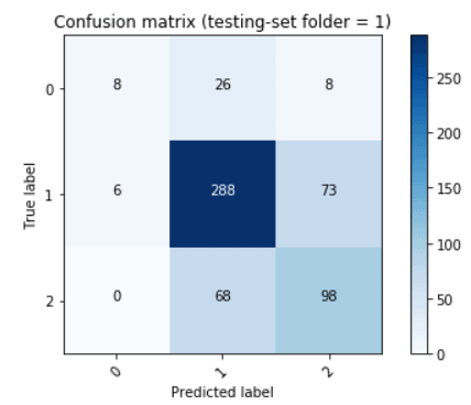
As you can see in the image above, the confusion matrix is a square matrix with one row and a column for each class in the classifier. The x-axis is used for the predicted values and the y-axis for the true values. Then a cell (i,j) in this matrix represents the number of predictions where the class j was predicted but the true class was the class i. Note that when i=j then cell(i,j) = cell(i,i) which are cells over the diagonal and represent the number of correct predictions that were done for the class i.
Some important metrics that we can calculate from the values in this matrix are:
- The overall accuracy (# of correct predictions / # total predictions)
- Precision for class i (# of correct predictions for class i / # total predictions for class i)
- Recall for class i (# of correct predictions for class i / # total true items in class i )
Also, since it’s easy to have a high recall with low precision and the opposite (high precision with low recall) it’s usual to add an F1 score metric (harmonic average of precision and recall) in order to combine precision and recall in just one metric, both being important to increase its value.
F1 = 2 x (precision x recall) / (precision + recall)
With this introduction to what a confusion matrix is, and the metrics that we can calculate, now let’s define a helper method to help us plot a pretty confusion matrix like the one in the image above. Later, after obtaining the final results we will see how to examine a confusion matrix and the metrics in more detail.
In [38]:
|
1 2 3 4 5 6 7 8 9 10 11 12 13 14 15 16 17 18 19 20 21 22 23 24 25 26 27 28 29 30 31 32 33 34 35 36 37 38 39 40 41 42 43 44 |
import itertools def plot_confusion_matrix(cm, classes, normalize=False, title='Confusion matrix', cmap=plt.cm.Blues): """ This function prints and plots the confusion matrix. Normalization can be applied by setting `normalize=True`. """ if normalize: cm = cm.astype('float') / cm.sum(axis=1)[:, np.newaxis] plt.imshow(cm, interpolation='nearest', cmap=cmap) plt.title(title) plt.colorbar() tick_marks = np.arange(len(classes)) plt.xticks(tick_marks, classes, rotation=45) plt.yticks(tick_marks, classes) fmt = '.2f' if normalize else 'd' thresh = cm.max() / 2. for i, j in itertools.product(range(cm.shape[0]), range(cm.shape[1])): plt.text(j, i, format(cm[i, j], fmt), horizontalalignment="center", color="white" if cm[i, j] > thresh else "black") plt.tight_layout() plt.ylabel('True label') plt.xlabel('Predicted label') def plot_confusion_matrix_with_accuracy(classes, y_true, y_pred, title, sum_overall_accuracy, total_predictions): cm = ConfusionMatrix(y_true, y_pred) print('Current Overall accuracy: ' + str(cm.stats()['overall']['Accuracy'])) if total_predictions != 0: print('Total Overall Accuracy: ' + str(sum_overall_accuracy/total_predictions)) else: print('Total Overall Accuracy: ' + str(cm.stats()['overall']['Accuracy'])) conf_matrix = confusion_matrix(y_true, y_pred) plt.figure() plot_confusion_matrix(conf_matrix, classes=classes, title=title) plt.show() |
Main method (k-fold cross-validation, with oversampling in training folders)
In [39]:
|
1 2 3 4 5 6 7 8 9 10 11 12 13 14 15 16 17 18 19 20 21 22 23 24 25 26 27 28 29 30 31 32 33 34 35 36 37 38 39 40 41 42 43 44 45 46 47 48 49 50 51 |
from sklearn.metrics import confusion_matrix from pandas_ml import ConfusionMatrix # K-folds cross validation # K=5 or K=10 are generally used. # Note that the overall execution time increases linearly with k k = 5 # Define the classes for the classifier classes = ['0','1','2'] # Make Dataset random before start df_rand = df.sample(df.storypoint.count(), random_state=99) # Number of examples in each fold fsamples = int(df_rand.storypoint.count() / k) # Fill folds (obs: last folder could contain less than fsamples datapoints) folds = list() for i in range(k): folds.append(df_rand.iloc[i * fsamples : (i + 1) * fsamples]) # Init sum_overall_accuracy = 0 total_predictions = 0 # Repeat k times and average results for i in range(k): #1 - Build new training and testing set for iteration i training_set, testing_set = rebuild_kfold_sets(folds, k, i) y_true = testing_set.storypoint.tolist() #2 - Oversample (ONLY TRAINING DATA) X_resampled, y_resampled = SimpleOverSample(training_set.label_title_desc.values.tolist(), training_set.storypoint.values.tolist()) #3 - train clf = FastTextClassifier() clf.fit(X_resampled, y_resampled) #4 - Predict y_pred = clf.predict(testing_set.label_title_desc.values.tolist()) #3 - Update Overall Accuracy for num_pred in range(len(y_pred)): if(y_pred[num_pred] == y_true[num_pred]): sum_overall_accuracy += 1 total_predictions += 1 #4 - Plot Confusion Matrix and accuracy plot_confusion_matrix_with_accuracy(classes, y_true, y_pred, 'Confusion matrix (testing-set folder = ' + str(i) + ')', sum_overall_accuracy, total_predictions) |


Evaluating the results
But, sometimes it’s not enough to use the overall accuracy. Suppose you have a dataset with datapoints divided into two classes, A and B. Suppose that 90% of the datapoints in your dataset belong to class A. Then you can create a dummy classifier that always predicts class A (without using any learning algorithm) and it achieves 90% accuracy! So, for that reason, other metrics like precision, recall or F1 score for each possible class could be helpful in scenarios like this (recall for class B in this example would have been 0, showing a clear problem predicting items of the minority class).
Having said this, we can take a look at the different confusion matrices that were generated in each iteration of our cross-validation process in order to average the important metrics to see how well our model performs for the different categories.
Class 0
- Average Precision for class 0: (12 + 8 + 9 + 10 + 8)/ (2 + 4 + 12 + 0 + 6 + 8 + 4 + 7 + 9 + 3 + 5 + 10 + 0 + 5 + 8) = 47/83 = 0.5663 (57%)
- Average Recall for class 0: (12 + 8 + 9 + 10 + 8) / (12 + 32 + 8 + 8 + 26 + 8 + 9 + 43 + 9 + 10 + 29 + 13 + 8 + 28 + 17) = 48/260 = 0.1846 (18%)
- Average F1 score for class 0: 2 x (0.5663 x 0.1846)/(0.5663 + 0.1846) = 0.2784
Class 1
- Average Precision for class 1: (281 + 289 + 267 + 273 + 270)/ (98 + 281 + 32 + 69 + 289 + 26 + 108 + 267 + 43 + 83 + 273+ 29 + 90 270 + 28) = 1380/1986 = 0.6949 (69%)
- Average Recall for class 1: (281 + 289 + 267 + 273 + 270) / (4 + 281 + 48 + 6 + 289 + 72 + 7 + 267 + 46 + 5 + 273 + 63 + 5 + 270 + 60) = 1380/1696 = 0.8137 (81%)
- F1 score for class 1: 2 x (0.6949 x 0.8137)/(0.6949 + 0.8137) = 0.7496
Class 2
- Average Precision for class 2: (90 + 97 + 82 + 96 + 97)/ (90 + 48 + 8 + 97 + 72 + 8 + 82 + 46 + 9 + 96 + 63 + 13 + 97 + 60 + 17) = 462/806 = 0.5732 (57%)
- Average Recall for class 2: (90 + 97 + 82 + 96 + 97) / (2 + 98 + 90 + 0 + 69 + 97 + 4 + 108 + 82 + 3 + 83 + 96 + 0 + 90 + 97) = 462/919 = 0.5027 (50%)
- Average F1 score for class 2: 2 x (0.5732 x 0.5027)/(0.5732 + 0.5027) = 0.5356
About precision
Precision for class X represents how good the model (classifier) is when it predicts that a data point belongs to class X.
We can see that the average precision for class 1 it’s close to 70% that means that 7 out of 10 of the class 1 predictions were predicted to be of class 1, the true value was predicted successfully. The other 30% were ‘confused’, mainly as items of class 2. You can repeat the same reasoning to see how the model performs when predicting class 0 and 2, achieving 57% precision in both classes, where the main confusion is items in class 1 – medium (in some way this could be expected, small sizes are confused with medium and some big are also confused with medium, but it’s good to have little confusion between small and big).
About recall
Recall for class X represents how good the model (classifier) is at finding data points that belong to class X.
We can observe that the main issue of our model is finding items from class 0 (small). Despite that almost 57% of the model’s predictions for class 0 are accurate, it still fails to give us as many predictions for class 0 as it should. For that reason, the average recall of class 0 is not as good as we’d like. On the other hand, our model is very good at finding class 1 (medium) items, successfully finding more than 80% of the items in that class. Finally, the recall for class 2 (big) allows us to see that our model is able to successfully find half of the items in class 2 (big), which is better than its recall for class 0 (small) but is not as great as its recall for class 1 (medium).
About the F1 score
The F1 score metric (harmonic average of precision and recall) allows us to combine precision and recall in just one metric, both being important to increase its value. So, since the F1 score for class 0 is much lower than the F1 score for class 2, which is lower than the F1 score for class 1, then we can validate that our previous observations are consistent and that our model performs very well at classifying items of class 1 (medium). It is also good at classifying items of class 2 (big) and although the precision at class 0 (small), suggests that we can trust quite well when the model predicts an item is small, we should note that a high percentage of the small items are not being found by our model. This is probably the first point to be improved upon in the future.
Building the application
|
1 |
ts = testing_set[["issuekey", "title", "description", "storypoint"]] #select only the columns to be serialized |
|
1 |
ts["prediction"] = y_pred # add predictions to the dataframe |
Later we used the “to_json” method as follows:
|
1 2 3 |
from IPython.html import widgets jsonDf = ts.to_json(orient='records') widgets.HTML(value = ''' backlog_items = ''' + jsonDf) |
Final thoughts on software development estimation
Some of the important things that we can conclude from this work are:
- Imbalanced datasets can be difficult to deal with in classification problems.
- The use of random downsampling did not achieve better results in our concrete problem.
- The use of a basic oversampling improved our results a bit. Some more complex oversampling techniques probably could get even better results and it’s something interesting to try out.
- The use of general pre-trained vectors for the English language from Wikipedia improved the results a bit, but not considerably.
- The use of more domain-specific pre-trained vectors from other open source repositories was better than using general pre-trained vectors, obtaining better results. It’s better to have few data but with good quality and very representative, than to have tons of data that are not representative of our domain or data with poor quality or noise.
- K-fold cross-validation is a helpful approach for model evaluation, mainly when the dataset is not too large as in our case
- Overall accuracy is important, but it’s not the only metric to be considered when evaluating a classifier. Metrics like Precision, Recall and F1 score can be a good option for evaluation metrics in classification problems.
We were able to train a model that could be taken as a base model from where to start and try to optimize it by tuning different parameters that need more experimenting. Other things that could help to improve the performance of our model is to use a smarter approach for oversampling and maybe the possibility of adding more real representative examples for the minority classes, in particular, more examples of small size items.
Also, it’s worth mentioning that if we are bad at estimating and the quality of the estimations in our dataset is poor, then the learning algorithm will probably have poor estimations as well. For this reason, something interesting to test would be to use a curated base history of items for training. That is, items that after having been done, the actual size (metric for the effort or how many hours they took) is added to the historical information.
Finally, although the results were not excellent, they were pretty good. We validated that a machine learning classification approach can be a good option for addressing the common yet difficult issue of estimating how complex a software development task is.
If you improve upon some of the results presented here, we’d love to know it! Also share your experience if you use some of these ideas to develop your own jira plugin to make your planning meetings more fun 🙂
About us
UruIT works with US companies, from startups to Fortune 500 enterprises, as nearshore partner for project definition, application design, and technical development. Our Uruguay and Colombia-based teams have worked on over 150 design and development projects up to date.
Are you ready to make the leap in your software development project? Tell us about your project and let’s talk!


1 comment